Lung Cancer Survival from synthetic EHR Data

Author

davechilders

Objective

This report demonstrates an end-to-end workflow for transforming synthetic EHR data into an analysis-ready dataset and performing a survival analysis on patients with lung cancer.

Specifically, this analysis:

ingests structured data derived from synthetic EHR records (Synthea)
constructs a patient-level dataset with time-to-event outcomes
applies survival analysis methods to estimate time from diagnosis to death

Data Source

Data for this analysis was generated using Synthea, a synthetic patient generator that produces realistic EHR-style records. The raw JSON output was processed into parquet files (patients, conditions, encounters) prior to this analysis.

The R code in this script can be viewed by clicking on Code.

The R script for turning synthetic EHR JSON data into tabular parquet files can be viewed on Github here.

Code

library(tidyverse)
library(fs)
library(arrow)
library(testthat)
library(scales)
library(survival)
library(lubridate)
library(gt)
library(survminer)

#dir_ls(glob = "*.parquet") %>% file_info() %>% select(path, size)

# load --------------------------------------------------------------------

cond <- read_parquet("conditions-2026-04-25.parquet")

pat <- read_parquet("patients-2026-04-25.parquet")
enc <- read_parquet("encounters-2026-04-25.parquet")

# data validation ---------------------------------------------------------

test_that("validation checks on patient_id", {
  
  expect_equal(
    cond %>% distinct(patient_id) %>% nrow,
    pat %>% distinct(patient_id) %>% nrow
  )
  
  expect_equal(
    cond %>% distinct(patient_id) %>% nrow,
    enc %>% distinct(patient_id) %>% nrow
  )
  
  expect_equal(
    cond %>% anti_join(pat, by = "patient_id") %>% nrow,
    0
  )
  
  expect_equal(
    cond %>% anti_join(enc, by = "patient_id") %>% nrow,
    0
  )

}
)

Test passed with 4 successes 🎉.

Data Transformation

To simplify joins across datasets, synthetic patient identifiers were replaced with sequential IDs. Date fields were also standardized for downstream analysis.

Code

# shorter patient IDs
pat <- pat %>% arrange(patient_id) %>% mutate(pid = row_number()) %>%
  select(pid, everything()) %>%
  select(-patient_id) %>%
  mutate(birthDate = as.Date(birthDate))

cond <- cond %>% 
  arrange(patient_id) %>%
  mutate(pid = dense_rank(patient_id)) %>%
  select(pid, everything()) %>%
  select(-patient_id)

enc <- enc %>%
  arrange(patient_id) %>%
  mutate(pid = dense_rank(patient_id)) %>%
  select(pid, everything()) %>%
  select(-patient_id)

Analysis Dataset Construction

The analysis dataset includes:

pid: patient identifier
cancer_onset: date of lung cancer diagnosis
death_date: recorded date of death (if applicable)
last_date: censoring date (death or end of observation)
outcome_days: time from diagnosis to last_date
onset_age: age at diagnosis
surv_obj: survival object combining time and event indicator

Patients were included if they had a recorded diagnosis of non-small cell lung cancer.

Code

cond_lung <- cond %>%
  semi_join(
    cond %>% filter(str_detect(tolower(condition_text), "lung cancer")),
    by = "pid"
  ) 

cond_lung2 <- cond_lung %>%
  mutate(
    lung_cancer = str_detect(tolower(condition_text), "lung cancer")
  ) %>%
  group_by(pid) %>%
  mutate(is_last = row_number() == n()) %>%
  ungroup() %>%
  filter(lung_cancer | is_last)

cond_lung_patient <- cond_lung2 %>%
  group_by(pid) %>%
  filter(any(condition_text == "Non-small cell lung cancer (disorder)")) %>%
  summarise(
    cancer_onset = onset_date[condition_text == "Non-small cell lung cancer (disorder)"],
    last_onset_date = onset_date[is_last],
    last_cond_death = as.integer(str_detect(tolower(condition_text[is_last]), "died"))
  ) %>%
  mutate(cancer_last_days = as.integer(last_onset_date - cancer_onset)) 

surv_df0 <- cond_lung_patient %>%
  left_join(
    enc %>%
      filter(encounter_type == "Death Certification") %>%
      select(pid, death_date = encounter_start),
    by = "pid"
  ) %>%
  select(-last_cond_death, -cancer_last_days) %>%
  mutate(
    death_outcome = ifelse(is.na(death_date), 0L, 1L),
    last_date = case_when(
      !is.na(death_date) ~ death_date, 
      TRUE ~ as.Date("2026-04-24")
      ),
    outcome_days = as.integer(last_date - cancer_onset)
    ) 

surv_df <- surv_df0 %>%
  left_join(pat %>% select(pid, birthDate, gender), by = "pid") %>%
  mutate(
    surv_obj = Surv(time = outcome_days, event = death_outcome),
    onset_age = time_length(interval(birthDate, cancer_onset), "year")
  )

head(surv_df) %>%
  select(pid, cancer_onset, death_date, death_outcome, last_date, outcome_days, onset_age,
         surv_obj) %>%
  gt() %>%
  tab_header(
    title = "Derived Analysis Data",
    subtitle = "First 5 rows"
  ) %>%
  fmt_number(onset_age, decimals = 1) %>%
  tab_footnote("Determined by condition of 'Non-small cell lung cancer (disorder)'",
               locations = cells_column_labels(columns = cancer_onset))

pid	cancer_onset¹	death_date	death_outcome	last_date	outcome_days	onset_age	surv_obj
Derived Analysis Data
First 5 rows
25	2008-11-02	2014-07-20	1	2014-07-20	2086	45.6	2086
186	2026-01-09	NA	0	2026-04-24	105	62.8	105+
214	2016-02-11	2019-09-12	1	2019-09-12	1309	50.2	1309
242	1982-05-02	1985-06-03	1	1985-06-03	1128	46.1	1128
266	2024-01-03	NA	0	2026-04-24	842	54.5	842+
320	1990-08-13	1994-12-10	1	1994-12-10	1580	47.5	1580
¹ Determined by condition of 'Non-small cell lung cancer (disorder)'

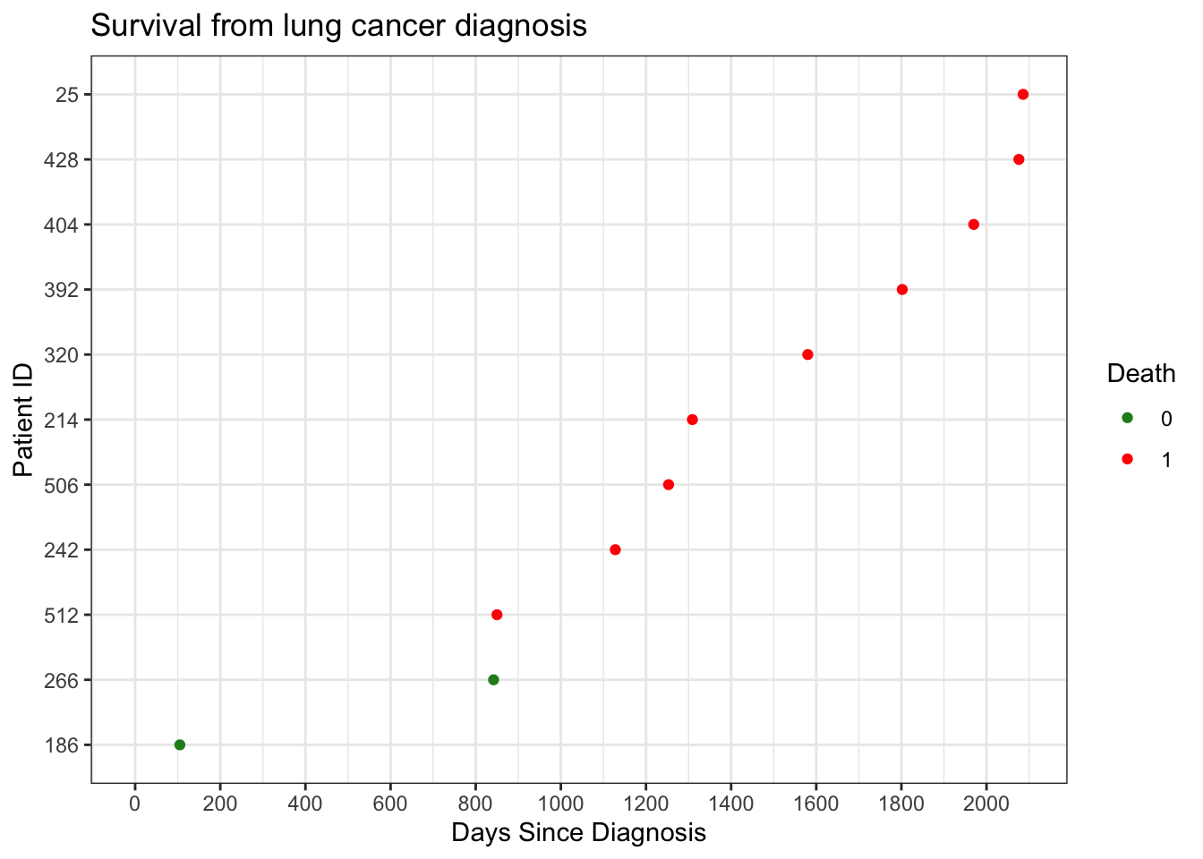
The plot below shows time from diagnosis to either death or censoring for each patient.

Key observations: - The cohort contains 11 patients - Time is measured relative to each patient’s diagnosis date (time zero) - With a small sample size, time to event fully separates observed outcomes

Code

# view survival outcomes 
ggplot(surv_df, aes(y = reorder(pid, outcome_days), x = outcome_days)) +
  geom_point(aes(color = factor(death_outcome))) +
  theme_bw() +
  expand_limits(x = 0) +
  scale_color_manual(values = c("0" = "forestgreen", "1" = "red")) +
  labs(
    title = "Survival from lung cancer diagnosis",
    x = "Days Since Diagnosis",
    y = "Patient ID",
    color = "Death"
  ) +
  scale_x_continuous(breaks = pretty_breaks(10))

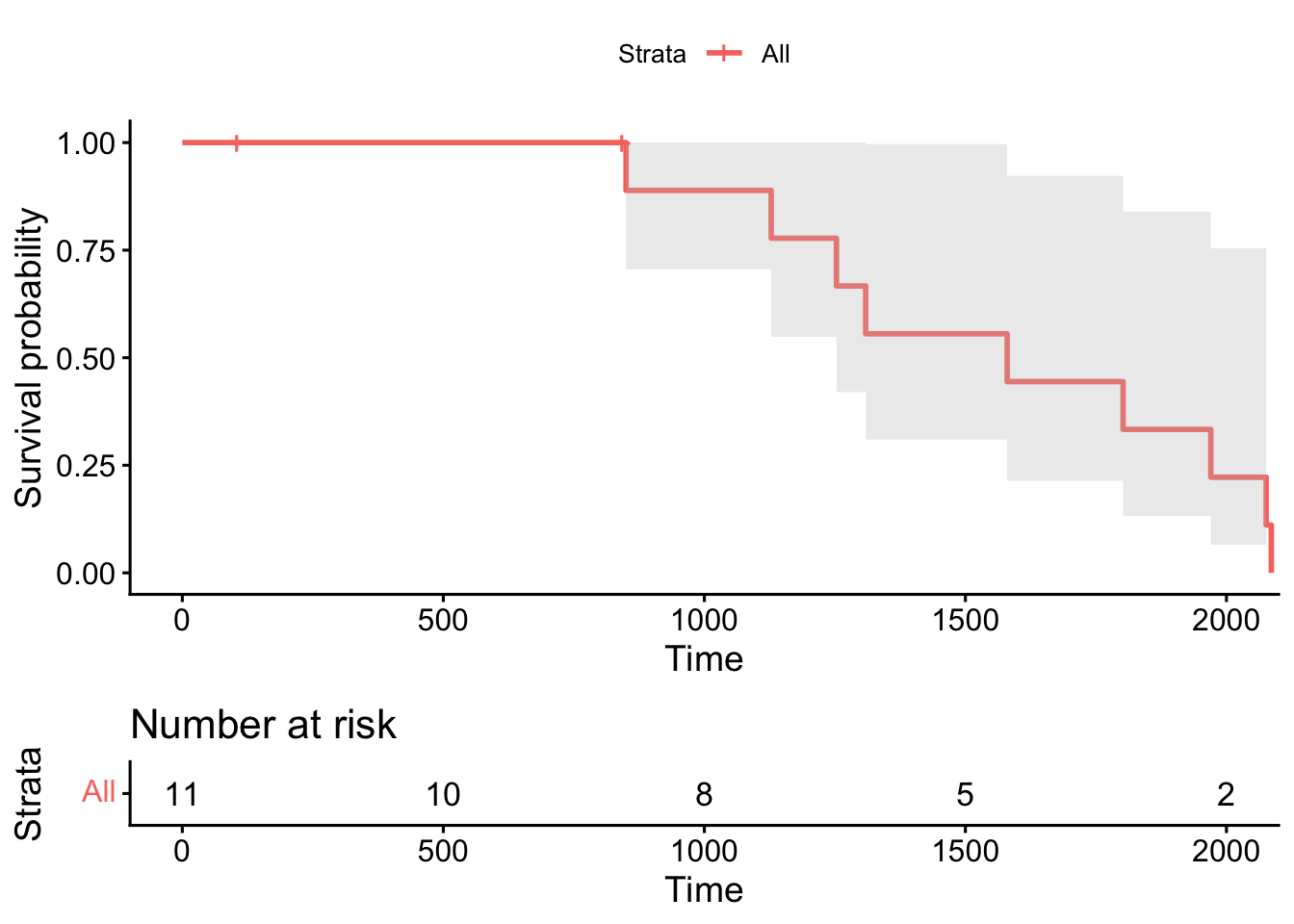
We will plot a Kaplan-Meier curve to show the survival probability against days since diagnosis.

Code

# kaplan meier curve
km_fit <- survfit(surv_obj ~ 1, data = surv_df)

#plot(km_fit, xlab = "Days", ylab = "Survival Probability", col = "blue", lwd = 2)

ggsurvplot(km_fit, data = surv_df, conf.int = TRUE, risk.table = TRUE)

Cox Proportional Hazards Model

It is not standard to fit a survival model with such a small sample size (n = 11). The model is included here for demonstration of workflow.

Here is the Cox PH model

\[h(t|x) = h_0(t)e^{\beta x}\] where:

\(x\) is age at onset
\(t\) is the days since diagnosis
\(h_0(t)\) is the unspecified baseline hazard function
\(\beta\) is the additive effect of age on the log-hazard

The hazard ratio for each unit increase in onset_age is obtained by exponentiating the coefficient:

Code

# age is only covariates
coxph_fit <- coxph(surv_obj ~ onset_age, data = surv_df)
coxph_output <- broom::tidy(coxph_fit, conf.int = TRUE, exponentiate = TRUE)

gt(coxph_output %>% 
     select(term, estimate, conf.low, conf.high, p.value)
   ) %>%
  tab_header(
    "Time to Death following Lung Cancer Diagnosis",
    subtitle = "Cox Proportional Hazards Model"
  ) %>%
  fmt_number(columns = estimate:p.value) %>%
  cols_label(
    term = "Covariate",
    estimate = "Haz Ratio",
    conf.low = "Lower 95% CI",
    conf.high = "Upper 95% CI"
  )

Covariate	Haz Ratio	Lower 95% CI	Upper 95% CI	p.value
Time to Death following Lung Cancer Diagnosis
Cox Proportional Hazards Model
onset_age	1.03	0.97	1.09	0.35

Interpretation

The hazard ratio represents the multiplicative change in the hazard of death associated with a one-year increase in age at diagnosis. Given the small sample size, estimates are primarily illustrative.